.AWS Timestream Best practices

For anyone looking for a fast, and scalable time-series database AWS Timestream is a great solution. It's serverless, provides quick analysis of data using SQL, has built-in analytics functions, can run millions of queries per day, scales on each layer (ingestion, storage, and query), and has data lifecycle management while remaining cost-effective.

In this blog post, I will cover Timestream optimizations and provide an example of the implementation for IoT data and the savings I managed to make using the methods described here.

⏳AWS Timestream introduction

What does AWS Timestream actually offer?

• AWS handled resource allocation
• Dynamic database schema
• Deduplication
• No maintenance/downtime
• Automatically added new features
• 99.99 SLA
• Up to 200 years of magnetic and 1 year in-memory storage
• Decouple architecture with automatic high availability across several availability zones
• AWS KMS encrypted by default

Let's take a look at the AWS Timestream architecture and its layers:

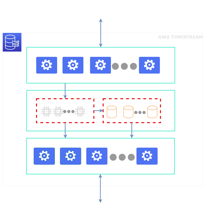
It consists of 3 independent layers, each scaling for itself:

• Ingestion layer - used to write data to the storage layer
• Storage layer - used to store data and consists of an in-memory and magnetic store
• Query layer - used to pull data using standard SQL from the storage layer

💰Pricing

With this understanding of how different layers scale, it is also important to understand how each layer is billed differently. This raises the complexity of calculations of Timestream pricing depending on how you use it.

It is important to note that, as of the time of writing this blog post, AWS Timestream is not included in the AWS Pricing calculator. Instead, AWS has pricing examples on the timestream web page as well as a convenient xlsx sheet.

⚙️ Pricing and Performance optimizations

If we dive deeper into the AWS documentation for Timestream we can get further insight into how each layer is billed and what are some of the key components to look out for when designing our database and making API calls to it.

Remember - this database is designed to be used for millions/billions of records and petabytes of data, so each optimization that you make counts and can create a huge impact on the overall performance and bill.

📝 Optimizing the Ingestion (Write) layer

This one can be a bit tricky, as there are several considerations to be made here, starting from the design of the database down to the column naming. Here are some quick tips and tricks:

• Batching - write data in batches, this will lower the amount of Write API calls and provide better response times
• Sort by time - timestream will have better write performance if your records are sorted by time
• Multi-measure records - use multi-measure records whenever possible instead of writing record by record (single measure records)
• Look for common attributes between data points
• Condense column names - you will get billed for column name lengths

📖 Optimizing the Query (Read) layer

The same things can be said about the Query API - it can get tricky to optimize queries.

• Query only columns that you need - avoid SELECT * statements and excess column queries as this affects scan times - this will benefit performance and pricing
• Use pagination - the SDK supports pagination, implement it for the best results
• Use functions - timestream has quite a bit of built-in functions available, use them!
• SQL support is sometimes inconsistent - it doesn't work exactly the same as standard SQL. For example, using the BETWEEN operator expects the min value to be first and max second, it will not work the other way around, even though it will in standard SQL
• Use time ranges - include time ranges in your queries to avoid excess data scanning

🏎️ Implementation and result

As promised, it's time to put my money where my mouth is... Or well, put my optimizations into practice and reap the benefits...

Let's take a look at the database model first. Our model supports up to 170 measures per IoT message, depending on the IoT device types, the size of this message can vary greatly, some devices have more sensors than others, but for this model, we have 3 device types.

For the sake of not diving too deep into our IoT devices, we can split the 3 device types into devices 1 through 3, with 1 having the least amount of sensors and 3 having the most amount of sensors.

An example structure of data at the entry point is given below:

Device3/Data/Hardware/Sensors/Values/Controller/Temperature
Device3/Data/Hardware/Sensors/Values/Controller/Voltage
Device3/Data/Hardware/Sensors/Values/Controller/Frequency

As you can already guess, this structure will simply be painful on your AWS bill if you try to flatten it and send it like this to the database. While a flat structure would be the easiest to map and understand, it would be the worse possible structure for performance and cost. In order to improve this the following naming scheme was used:

Dvc3_CtrlTemp
Dvc3_CtrlVolt
Dvc3_CtrlFq

Now, this is much better, it's kept short enough not to harm our performance/billing and long enough to be easily understandable. These optimizations were applied across all 3 device types, and in turn, the original vs shortened naming is now much lighter.

As you can see, the more complex the data structure is, the more you save by optimizing it.

Ok, so we have our database schema worked out and shortened, now it's time to work on our write-api improvements.

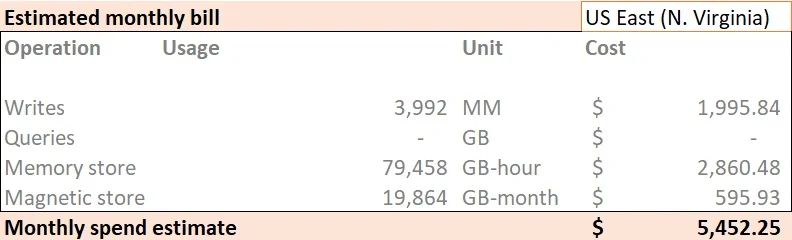
Based on the table above, our average IoT message size is about 1.85KB, on the gateway (not on the database side), with an average of 100 measures - assuming we have an equal amount of all 3 types of devices deployed. So, let's do some math, with the help of the pricing xlsx sheet to calculate how much it will cost to write all of this data. We have about 220 IoT messages per second incoming on the API which we plan to store for 24h in-memory storage and 6 months in magnetic storage. The billing will be shown for write-api and storage costs as well.

Using the xlsx sheet, this is what we got for single measure records with no batching enabled:

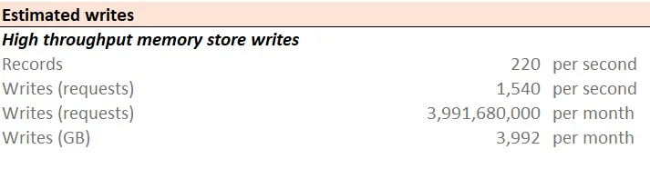
Which equates to the write + storage bill of:

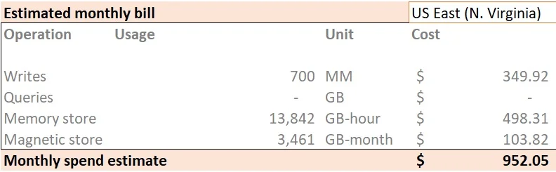
Now, what will happen if we use multi-measure records with batching enabled (50 records per batch):

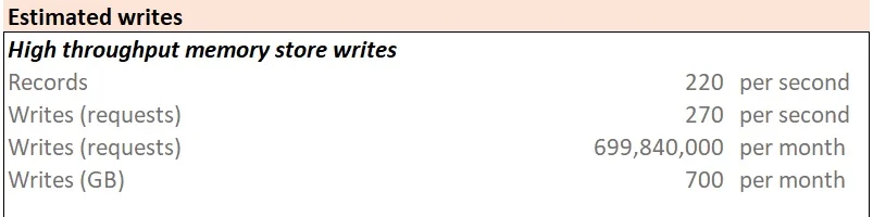
Which equates to the write + storage bill of:

Wow, now this is some drastic improvement. Further improvements can be made using common attributes, however, for the implementation above it doesn't make a lot of sense since we don't have many (if any at all) common attributes when working with our IoT data setup.

But let's take a look at an example of where it makes sense, so for that purpose AWS's example (AWS Online Tech Talks) using EC2 metrics is perfect.

In this example, AWS EC2 metrics are collected -

• time - timestamp value
• region - us-east-1
• az - 1d
• hostname - host-24Gju
• cpu_utilization - 35.0
• mem_utilization - 54.9
• network_bytes - 30000

The calculations provided are just for write-api costs, excluding storage costs. Let's take a look at the costs from the video:

Single-measure records with no batching enabled: 25.92$
Single-measure records with batching enabled: 2.85$

Now, analyzing the data structure, you can see that there will be quite a bit of data in common - region, az, hostname, and VPC. This is a perfect example of the type of data you want to put in the common attributes. Once set up, this is the end result:

Single-measure records with common attributes and batching enabled: 0.78$

For the full breakdown of the data and calculations please watch the video as it is a deep dive into Timestream and will provide valuable insight.

🚀 Conclusion

AWS Timestream is an extremely powerful time-series database designed to handle terabytes of data ingestion per day with new and amazing features continuously being added - AWS re:Invent 2021 session. With these features and improvements, it is more than competitive against existing time-series solutions, and with proper implementations on the write and query side of the API, performance and especially billing will be amazing as well. During development, using batch operations in the write-api our IoT data ingestion improved response times by up to 133% (5x faster).

In the following months as new features and improvements are added, we will keep writing about them and testing them out. In the meantime, check out the rest of our tech blog!